|
|
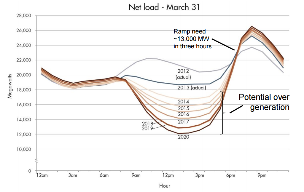
| Fig. 1: CAISO's 2013 illustration of the "duck curve," in which net load is plotted versus the time of day for a particular California spring day. The significant drop during midday (the duck's back) is caused by the large power input from solar resources. Predictions for different years are included on the graph; this article examines the estimated 2015 net load. [1] (Courtesy of CAISO) |
California Independent System Operator (CAISO)'s "duck curve" illustration (see Fig. 1) shows the challenge of integrating intermittent resources like wind and solar power into our existing infrastructure and consumption habits. Energy storage will likely play an important role in the successful integration of renewable resources, in conjunction with other improvements and efficiency boosts to multiple layers of the power system. As a simple thought experiment, this article roughly estimates the capital cost and scale required to "fix" the intermittency problem on a daily basis through energy storage alone.
California Independent System Operator (CAISO) is an independent organization that operates the power grid serving most of California. In other words, CAISO is the entity responsible for coordinating electricity generation and transmission across the state, and for forecasting electricity demand in the near future in order to ensure sufficient generation is achieved. While CAISO itself is not responsible for generating power for the grid, it oversees the energy production market and is charged with securing enough power to satisfy California's electricity demand at any given time.
As renewable energy resources (primarily wind and solar) achieve higher market penetration, they present a new problem for CAISO and other independent system operators: because many of these energy sources are inherently intermittent, the amount of power that must be generated by conventional plants will become more variable on an hourly basis. For instance, solar power generation occurs during daylight hours, meaning conventional power generation doesn't need to produce as much power around midday as during the nighttime. Intermittent resources like wind and solar power are called variable generation resources.
|
|||||||||||||||||||||||||||||||||||||||||||||||||||||||||||||||||
| Table 1: Estimated net load values for 2020 from CAISO's "duck curve" image (Fig. 1). Data acquired by tracing the original CAISO graph with ~20 MW precision. |
This situation is the basis of the problem shown in the so-called "duck curve." Because variable generation resources like solar power significantly reduce the load on conventional generators during the day but not during the night, a surge in generation demand may occur as the sun sets. This trend is shown in Fig. 1. [1] Plotted against the time of day is the net load, which is defined as the total load on the power grid (i.e. power demand from consumers) minus input from variable generation resources (i.e. wind and solar). [1] The plot depicts hourly net load for a certain March 31st day, with different net load predictions provided for each year through 2020. The plot is said to resemble certain species of waterfowl because of the high peak on the right (the head), drooping midsection (the back), and taller left side (the tail).
Note that CAISO does not specify how they produced the hourly net loads shown in the "duck curve" image, nor under what conditions the hourly net loads were modeled. (Some accuse CAISO of using a worst-case scenario for the spring day in which clear, sunny skies boost solar production while cold temperatures increase nighttime heating demand to exaggerate the curve's steepness. The political motivations for this debate are complex and worth researching.) CAISO also does not provide the exact net load values plotted in the image; for the purposes of this article, the 2020 net load curve was traced to estimate CAISO's hourly net load values (see Table 1).
The high variability in net load seen in the duck curve scenario is problematic because much of California's conventional generators require long periods of time to start or stop producing power. [1-4] Because of these long startup times, power generation cannot easily be scaled down during the midday drop in net load and reinstated in time for the post-sunset jump. In addition, some non-dispatchable generation sources such as nuclear power, geothermal power, cogeneration, and hydropower at minimum production levels cannot be shut off temporarily or set to produce less than a certain power (see Fig. 2). According to testimony given to the FERC, CAISO's minimum non-dispatchable power production is about 15,000 MW - meaning the power grid's online generators cannot produce less than 15,000 MW at any one time. [4]
 |
| Fig. 2: The 2020 duck curve superimposed on a breakdown of CAISO's non-dispatchable resources. Note the 15,000 MW non-dispatchable generation value. [4] (Courtesy of CAISO) |
In CAISO's 2020 duck curve scenario, the net load drops well below 15,000 MW during the hours of peak sunlight (see Fig. 1). This presents an overgeneration risk, in which the system's power demand is lower than the minimum power production possible. [1,4] During overgeneration conditions, the excess supply of power could potentially damage generators and motors connected to the grid, so system operators normally monitor demand to closely match power production. [2] But since the 2020 duck curve scenario drops below the minimum generation of 15,000 MW, CAISO would instead be forced to implement curtailment, in which variable generation sources like wind and solar are scaled back to keep the net load above the minimum generation value, or implement negative electricity prices to force net load upwards. [2,4] As curtailment nullifies the zero-emission benefits of solar and wind power, it is generally an unfavorable option.
In summary, the primary problems presented by the duck curve are the risk of overgeneration during the middle of the day, and the steepness of the load increase during the late afternoon and evening. Going forward, this article will examine energy storage as a solution to these problems by storing excess power production from the day and using it during the night, thereby eliminating overgeneration risk and consequentially flattening the late-day increase to an extent.
Load balancing refers to the redistribution of the aforementioned variability in net load, in essence making the net load plot flatter. The rest of this article examines how California could use energy storage alone to mitigate the ramping and overgeneration problems presented above. In other words, how much physical storage would be needed for each technology, and how much would it cost? Using the values from Table 1 and simple trapezoidal-rule calculations, this article evaluates two scenarios for the above March day in 2020, both described below:
 |
| Fig. 3: Illustration of using energy storage to capture energy during overgeneration risk period (colored green) and discharging said energy during peak net load hours (colored red). (Base Image from Bouillon. [4]) |
The immediate problem presented by the duck curve is the risk of overgeneration during the middle of the day, as the net load falls significantly below CAISO's minimum generation of 15,000 MW. So for the first, less-ambitious scenario, all energy production that occurs while the net load lies below the 15,000 MW limit is stored and discharged at the evening peak in net load. In this scenario, the peak charge rate of the energy storage would be 2,290 MW (at 1:30 pm); the total energy storage needed would be roughly 13,720 MWh; and the maximum discharge rate would be roughly 4,820 MW (at 8:30 pm). (See Fig. 3).
To get an idea of the largest-possible scale of a grid-wide storage project, the second, more ambitious/unrealistic scenario aims to completely flatten the net load to the day's average of roughly 18,340 MW. Here, the peak charge rate of the energy storage would be roughly 6,260 MW (at 1:30 pm); the total energy storage needed would be roughly 39,897 MWh; and the maximum discharge rate would be roughly 20,300 MW (at 8:30 pm). While this scenario would clearly never actually come to fruition, given the difficulty of forecasting net load and the lack of benefits from completely flattening the curve, it provides an upper limit to the energy storage proposal. (See Fig. 4).
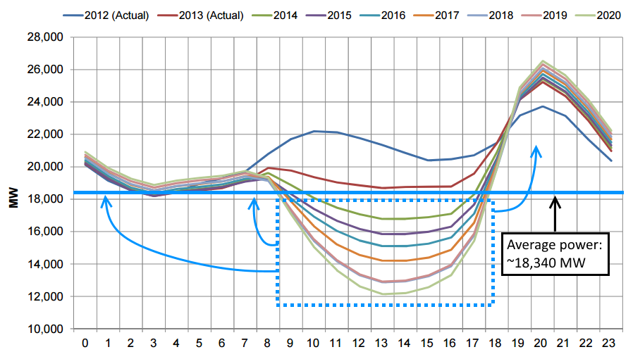 |
| Fig. 4: In the second scenario, the entire day is load-balanced so that net load is completely flat at the day's average of ~18,340 MW (shown as blue line). Excess power produced while net load is below 18,340 MW is stored and supplied to the grid whenever net load is above 18,340 MW. (Base image from Bouillon. [4]) |
Here we give a cursory look at the scale and cost needed to tackle each of the above scenarios with eleven different energy storage technologies. Average capital cost per MW/MWh for each technology, as well as other technical aspects listed, are sourced from a recent review by Zakeri and Syri, with Euro amounts converted to USD at the May 2014 exchange rate of 1.36 Euros/USD. [5] The storage mediums examined include mechanical (pumped hydropower storage, compressed air (above and belowground)), conventional battery (lead-acid, sodium-sulfur, nickel-cadmium, sodium-nickel chloride, lithium-ion), flow battery (vanadium, zinc-bromide), and hydrogen fuel cell technologies. (See Table 2).
For both scenarios, we assume charge rate and discharge rate are roughly the same, meaning we can focus on the higher discharge rates when examining power capacity. [6]
According to these rough calculations, the total initial capital needed to set up sufficient energy storage for scenario 1 ranges from about 5 to twenty billion USD, while scenario 2 entails about 25 to 95 billion USD. While these financial figures are quite large, especially given the underestimation of the cost of infrastructure and maintenance, they are not otherworldly considering the problem they (perhaps too ambitiously) solve. Interestingly, the three mechanical storage technologies (pump hydropower, CAES) and flow batteries came out as the cheapest routes, beating out some electrochemical technologies with larger realized scales than aboveground CAES and flow batteries. Pumped hydropower storage and belowground CAES are expectedly among the cheapest, as they are by far the most established energy storage mediums worldwide. Aboveground CAES is still being prototyped and developed, and is more difficult on a large scale than belowground CAES because of the additional costs of construction. [5] This explains its smaller realized scale but lower capital costs when compared to the other more established mechanical energy storage methods. Flow batteries, while supposedly cheap, still have a long ways to go before becoming truly scalable and commercially viable for large projects (as evidenced by their small realized scales).
|
||||||||||||||||||||||||||||||||||||||||||||||||||||||||||||||||||||||||||||||||||||||||||||||||
| Table 2: Total capital costs (TCC) and costs of implementing each scenario for each technology. [5] CAES = Compressed Air Energy Storage. ZEBRA = Zero Emission Battery Research (sodium-nickel chloride). "Efficiency" refers to the energy that can be discharged from the storage system divided by the energy originally put into the system. "Realized scale" provides an example of one of the largest individual storage projects of each technology that is or has been fully operational. Technical and project details sourced from Zakeri and Syri unless otherwise noted. [5] |
One must note that the cost analysis involved in the above numbers introduces immense complexity and uncertainty. In the words of Zakeri and Syri:
"Estimating the cost of EES [electric energy storage] systems includes levels of uncertainty and complexity. Except of some mature technologies, the use of large-scale EES systems is scarce and the economic performance of the existing sites is not widely reported in the literature. The cost data are scattered, from different times and power markets, and calculated/estimated based on different methods. Since most of the EES technologies are in the early stages of development and demonstration, their cost data cannot be conveniently scaled for the larger or smaller sizes." [5]
Many of these technologies are unproven, or have problems not easily accounted for in basic cost analyses (e.g. environmental damage, material scarcity, lack of infrastructure, etc.). [12] The study also found that some technologies had much greater variability in cost than others. In addition, the total capital cost (TCC) figures do not account for ongoing operation and maintenance, sub-optimal efficiencies, or for differing lifecycle spans and replacement costs. [5] To try and accommodate these uncertainties, various other technical and contextual details are provided in the Table 2. No single technology out of the above eleven will independently solve the intermittency problem of renewable energy; the above calculations are simply meant to provide ballpark numbers and a sense of scale for such a project.
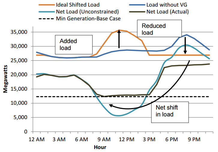 |
| Fig. 5: A figure from Denholm et al. showing the "flattening" of the duck curve through shifting demand, similar to Scenario 1 in this article. [2] Some values from Denholm et al. differ than those used in this article (e.g. minimum generation) due to more complex analysis. (Courtesy of the U.S. Department of Energy) |
Upgrading California's power grid to accommodate the increasing penetration of renewable, variable generation resources will surely be a multi-faceted effort: many geographic and temporal grid flexibility strategies can be applied to the power system to help alleviate the problems exemplified by the duck curve in both the short term and long term. [2] Energy storage will likely play an important role in future improvements to power systems, as they allow operators to effectively redistribute energy supply and demand to the optimal times. In fact, a detailed 2015 NREL report by Denholm et al. produced a similar solution to the above Scenario 1, but with other grid improvements included in the simulation (see Fig. 5). [2] This report is well worth reading for anybody interested in the duck curve and the intermittency problem in general. Another report by the Vermont-based Regulatory Assistance Project analyzes a diverse array of strategies to combat the problems posed by the duck curve, concluding that technologies available today are sufficient to mitigate both the steep ramping problem and the overall disparity in net load between peak and minimum hours. [3]
The simple cost comparison above shows that even immense storage projects (such as using storage alone to remove overgeneration and curtailment, as in Scenario 1 above) are within the financial realm of feasibility. Especially when considering energy storage as just one of many strategies to improve renewable energy penetration, several of the examined technologies show promise. In the words of Denholmm et al. on the duck curve, "a relatively small amount of storage [...] could provide significant benefits across the entire Western Interconnection." [2] Pumped hydropower storage - by far the most established storage technology - is still among the most cost-effective and efficient storage mediums; while compressed air energy storage shows immense promise for future scalability. Several electrochemical technologies also show promise and modest real-world realization, and will most likely become key components to the future of power systems. While widespread energy storage still faces a variety of challenges, a thorough mix of the above storage technologies, as well as many other grid flexibility improvements, will likely be the key to successful integration of renewable resources in the future. [2,6,12]
© Michael Burnett. The author grants permission to copy, distribute and display this work in unaltered form, with attribution to the author, for noncommercial purposes only. All other rights, including commercial rights, are reserved to the author.
[1] "What the Duck Curve Tells us about Managing a Green Grid," California Independent System Operator, October 2013.
[2] P. Denholm et al., "Overgeneration from Solar Energy in California: A Field Guide to the Duck Chart," U.S. National Renewable Energy Laboratory, NREL/TP-6A20-65023, November 2015.
[3] J. Lazar, Teaching the 'Duck' to Fly, Second Edition," Regulatory Assistance Project, February 2016.
[4] B. Bouillon, "Prepared Statement of Brad Bouillon on Behalf of the California Independent System Operator Corporation," U.S. Federal Energy Regulatory Commission, 10 Jun 14.
[5] B. Zakeri and S. Syri, "Electrical Energy Storage Systems: A Comparative Life Cycle Cost Analysis," Renew. Sust. Energy Rev. 42, 569 (2014).
[6] J. Eyer and G. Corey, "Energy Storage for the Electricity Grid: Benefits and Market Potential Assessment Guide, Sandia National Laboratories, SAND2010-0815, February 2010.
[7] "Wind Firming EnergyFarm," Primus Power, October 2012.
[8] "INGRID 39 MWh Grid-Connected Renewable Energy Storage Project," Fuel Cells Bulletin, 2012, No. 8, 9 (2012).
[9] B. Bollinger, "Technology Performance Report: SustainX Smart Grid Program," SustainX, 2 Jan 15.
[10] M. Budt et al., "A Review on Compressed Air Energy Storage: Basic Principles, Past Milestones and Recent Developments," Applied Energy 170, 250 (2016).
[11] Pumped Storage and Potential Hydropower from Conduits," U.S. Department of Energy, February 2015.
[12] C. J. Barnhart and S. M. Benson, "On the Importance of Reducing the Energetic and Material Demands of Electrical Energy Storage," Energy Environ. Sci. 6, 1083 (2013).