|
|
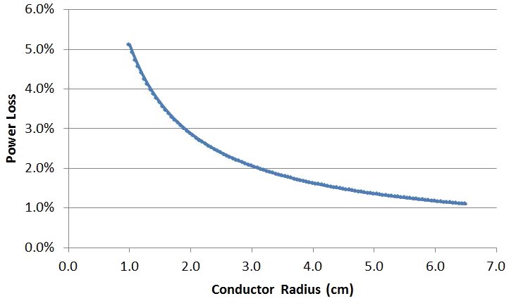
| Fig. 1: Resistive Loss on a Al transmission line as a function of radius as a percentage loss over 1000 km. |
According to the Department of Energy, California lost about 19.7 x 10⁹ kWh of electrical energy through transmission/distribution in 2008. [1] This amount of energy loss was equal to 6.8% of total amount of electricity used in the state throughout that year. At the 2008 average retail price of $0.1248/kWh, this amounts to a loss of about $2.4B worth of electricity in California, and a $24B loss nationally. [1] This report looks to explain and quantify the two major sources of loss in high voltage AC transmission lines: resistive loss and corona loss. The former occurs because of the non-zero resistance found wire's metal. Corona loss is an ionization of the air that occurs when the electric fields around a conductor exceed a specific value.
Although the conductors in a transmission line have extremely low resistivity, they are not perfect. This section seeks to quantify that loss through computation of the skin depth and power attenuation factors.
The amount of resistive loss in a system can be found estimated by using corona-free transmission line equations to find the amount of power delivered to any point along the wire and subtracting the initial amount of power. The equations for doing so are below: [2]

In the above equation, c is the speed of light and L, the inductance per unit length of the transmission line is given as:
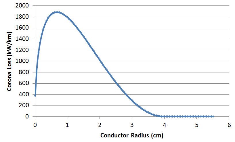 |
| Fig. 2: Corona loss in kilowatts lost per kilometer of wire as a function of radius. An Al 3 phase 765kV transmission line and Peek's formula were used to generate this graph. |
The equations for calculating Rl, the resistance per unit length, can be shown below. It includes the formula for finding the wire's skin depth (δ), which shows how far into the conductor 90% of the power is carried by current. [3]
IB in this equation is correction factor found by using the first two Bessel I functions.
Using the above equations, the total amount of power lost due to resistance is equal to the power at a given distance minus the inital power. Since the amount of loss as a percentage is a fixed amount regardless of initial power, the results listed are written as a percentage of total power. The parameters listed above and summaries of the results of these equations can be found in Table 1. In it, there are estimated losses of a typical US power line made of aluminum (Case 1), a European power line at 50Hz (Case 2), and a line made out of silver (Case 3). A comparison of cases 1 and 3 show that building a long transmission cable can save in resistance loss (about $19M/year), but would cost significantly more to build ($18.5B) at 2010 market prices.
|
||||||||||||||||||||||||||||||||||||||||||||||||||||||||||||||||||||||
| Table 1: Resistive loss values using sample parameters and the formulas listed above. | ||||||||||||||||||||||||||||||||||||||||||||||||||||||||||||||||||||||
In a paper from the American Electric Power (AEP) company published in 1969, the authors make an estimate that the amount of power loss from non-corona based effects is about 4MW over 100 miles in a 1GW transmission system. [7] Converting to metric units, this gives a loss of about 25MW or 2.5% over a 1000km transmission line. This number is consistent with the resistive loss given in a contemporary, self-published report from the AEP. [11] In this report, the resistive loss was listed as between 3.1MW/100 miles and 4.4MW/100 miles, depending on the wiring configuration. This corresponds to between a 1.9% and 2.8% power loss over 1000km.
Corona loss is the other major type of power loss in transmission lines. Essentially, corona loss is caused by the ionization of air molecules near the transmission line conductors. These coronas do not spark across lines, but rather carry current (hence the loss) in the air along the wire. Corona discharge in transmission lines can lead to hissing/cackling noises, a glow, and the smell of ozone (generated from the breakdown and recombination of O2 molecules). The color and distribution of this glow depends on the phrase of the AC signal at any given moment in time. Positive coronas are smooth and blue in color, while negative coronas are red and spotty. [5] Corona loss only occurs when the line to line voltage exceeds the corona threshold. Unlike resistive loss which where amount of power lost was a fixed percentage of input, the percentage of power lost due to corona is a function of the signal's voltage. Corona discharge power losses are also highly dependent on the weather and temperature.
The corona factor equation was empirically derived by F.W. Peek and published in 1911.[4] In a later publication, he modified the original equation and he showed that the total amount of power loss in a wire due to the corona effect was equal to the equation below: [5]
For examples of these values and their meaning, please refer to Table 2.
|
||||||||||||||||||||||||||||||||||||
| Table 2: Sample corona loss calculation based on Peek's formula. | ||||||||||||||||||||||||||||||||||||
As can be seen in Fig. 2, the radius of the conductor has a large effect on the total amount of corona loss. One way of getting lines with a larger effective radius is through the use of bundles, where 2-6 separate, but close lines are kept at the same voltage via intermittent connectors. This reduces the amount of metal needed to achieve a given radius and corona loss. Transient calculations of corona loss can be found in reference [10].
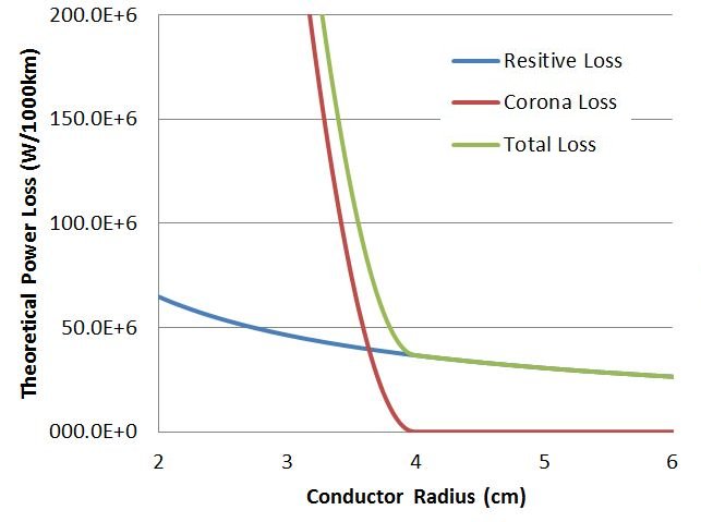 |
| Fig. 3: Total loss of a 2.25 GWm 3 phase 765 kV transmission line as a function of radius. |
In reference [6], the authors measured the corona loss of a 765kV, 3 phase, and bundled transmission line to be about 1.87kW/km in fair weather. This amounts to only about a 0.083% loss over a 1000km line. In bad weather, however, the authors measured the loss to be 84.3kW/km, or about a 3.7% loss. Using these numbers and the average price of electricity, a day long rainstorm on a 100km stretch of 765kV wires costs an electric company about $25,000.
Looking at voltages greater than 765kV, the Hydro-Quebec Institute of Research measured the amount of corona loss at voltages up to 1200 kV. [8] They found that the corona loss of a 6 and 8 conductor bundles were 22.7 kW/km and 6.2 kW/km, respectively. These numbers were measured in "heavy artificial rain". The discrepancies between [6] and [8] probably stemmed from different radii and conductor spacing.
Finally, researches in Finland measured the amount of corona loss in transmission lines under frost conditions. [9] This paper also shows the large reduction in corona loss from bundling wires: about 2.5-5x for each conductor added between 1-3. Under frost conditions, they show that the loss of the lines is about 21 kW for a 2 conductor bundle of a 400kV three phase transmission line.
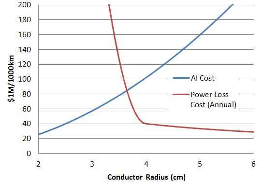 |
| Fig. 4: Cost of a 2.25 GWm 3 phase 765 kV transmission line as a function of radius. The cost of a transmission line was found by taking the total wire volume and multiplying by the 2010 market price of aluminum ($1.14 per pound). |
This report shows the how to estimate both corona and resistive losses in wire and also gives experimental results. Fig. 3 provides an estimate of the total amount of loss in a system as a function of the conductor radius. Looking at this figure, the amount of loss drops dramatically as the wire radius increases to about 4cm. If made of solid metal (as the formulas above assume), this would be a fairly unwieldy size. Because of this, power line companies bundle smaller lines to keep both building and loss costs as low as possible.
Fig. 4 shows the total amount of theoretical power loss and cost of a 1000km high voltage transmission line. As the wire gets larger, the amount of loss decreases as about 1/r (resistive) and quadratically to 0 (corona). Larger wires also incur a quadratically larger cost, and eventually reach a break-even point where larger conductor radii do not make financial sense. It should be noted that this figure (wrongly) assumes a solid, homogeneous wire. Power lines, in addition to being bundled, also contain a cheaper steel core on the interior of the wire. This is because once past the skin depth into the wire, where 90% of the power is carried, the resistivity of the wire becomes less important.
© 2010 C. Harting. The author grants permission to copy, distribute and display this work in unaltered form, with attribution to the author, for noncommercial purposes only. All other rights, including commercial rights, are reserved to the author.
[1] M. Bowles, " State Electricity Profiles 2008," US Energy Information Administration, DOE/EIA 0348(01)/2, March 2010.
[2] W. Hayt and J. Buck, Engineering Electromagnetics (Mcgraw-Hill, 2006), pp 346, 486.
[3] F. Rachidi and S. Tkachenko, Electromagnetic Field Interaction with Transmission Lines From Classical Theory to HF Radiation Effects (WIT Press, 2008).
[4] F. W. Peek, "The Law of the Corona and the Dielectric Strength of Air," Transactions of A.I.E.E. 30, 1889 (1911).
[5] F. W. Peek, Dielectric Phenomena in High-Voltage Engineering (McGraw-Hill, 1929), pp 169-214.
[6] N, Kolcio et al., "Radio-Influence and Corona-Loss Aspects of AEP 765-kV Lines" IEEE Transactions on Power Apparatus and Systems PAS-88, No.9, 1343 (1969).
[7] G. S. Vassell and R. M. Maliszewski, "AEP 765-kV System: System Planning Considerations" IEEE Transactions on Power Apparatus and Systems PAS-88, 1320 (1969).
[8] N. G. Trinh, P. S. Maruvada and B. Poirier, "A Comparative Study of the Corona Performance of Conductor Bundles for 1200 kV Transmission Lines," IEEE Transactions on Power Apparatus and Systems PAS-93,940 (1974).
[9] K. Lahti, M. Lahtinen and K. Nousiainen, "Transmission Line Corona Losses Under Hoar Frost Conditions," IEEE Transactions on Power Delivery 12, 928 (1997).
[10] X. Li, O. Malik and Z. Zhao, "Computation of Transmission line Transients Including Corona Effects," IEEE Transactions on Power Delivery 4, 1816 (1989).
[11] " Transmission Facts," American Electric Power.