 |
 |
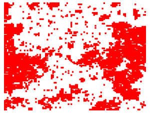
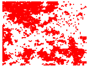
| Fig. 1: An example of a block-spin transformation in the critical Ising model. Coordinates of blocks for statistically equivalent distributions is produced by the code here. |
The Ising Model is a simple description for the magnetic interaction of an array of spins. It has been known for some time that, at the critical temperature, the model exhibits scale-invariance. This property renders the system exactly solvable. As a demonstration of the power of conformal invariance, we will calculate and display the 2-point correlation function for a toriodal geometry.
The Ising Model describes a collection of spins, s, interacting with a nearest neighbor coupling J. The Hamiltonian, or energy function, is given by

where the sum is taken over nearest-neighbor lattice sites, and J is the reduced coupling constant, inversely proportional to the temperature. Because of the overall minus sign, spins tend to line up parallel to each other. Indeed, the zero-temperature ground state simply consists of all spins pointing in the same direction. If we raise the temperature slightly, however, thermal fluctuations will force the configuration of spins to depart from uniformity. For very low temperatures, the majority of the spins will still be aligned. In experimental terms, the sample will have a net magnetization. If the temperature is high, however, thermal fluctuations will completely destroy the system's order, and the spins will be evenly distributed up and down, with zero net magnetizaion. At some intermediate temperature, the "critical temperature", or Tc, the Ising system undergoes a phase transition.
Precisely at the critical temperature, the Ising model exhibits several interesting behaviors, including the property of scale invariance. This concept can be described in many ways: stated simply, scale invariance means that a configuration of spins looks the same at all levels of magnification. More formally, it means that if we trace out the short length degrees of freedom in the partition function, the hamiltonian for the remaining degrees of freedom will be precisely the same as the original H, with an identical coupling. Equivalently, the critical Ising model defines a fixed point of the Renormalization Group.
This phenomenon can be seen at work in the figures at left. The top figure represents a typical configuration of spins in the critical Ising model. Solid squares represent lattice sites with spin up, and blank squares represent sites with spin down. If we "put on blurry glasses," and group each block of 9 spins together as one unit, either up or down, according to the majority of the individuals within the block, we can form a new configuration of spins. The bottom figure is the result of applying this process to the top. You can see the original configuration, smaller and slightly "blurred," in the lower left corner of the second image. The distribution of cluster sizes in the two systems looks strikingly similar. The exact scale invariance of the critical Ising model ensures that they are statistically identical, in the sense that they each have equal probabilities.
Scale invariance of the critical Ising model can be made rigorous (see the Appendix report for a partial review of the evidence). For simplicity, however, we will instead assume scale invariance (motivated by the statisticaly similarity of the two figures), and see what we can derive. Specifically, let's see what constraints this invariance imposes on correlation functions. The correlation function is defined as the expectation value of the product of two spins, separated by distance r:

Suppose that we perform a Renormalization Group transformation with scale factor b. This is equivalent to grouping together a block of spins, with b spins on each side, into a single unit. Let's consider a correlation function between two of these units, r blocks apart. In the blocked system, this is a simple two-point correlation function, G(r). But we can also write the correlator of the blocks in terms of correlations of individual sites in the original system that make up the blocks. Specifically, this correlator will consist of correlation functions between the sites in block A and the sites in block B, multiplied by a complicated factor accounting for the number of spins in each block, and the interactions between them. Crucially, this factor is insensitive to the distance between the blocks, it can only depend upon the scaling parameter b. We write this statement as G(r) = f(b)G(br). Now,consider compounding two spin-blocking transformations, one with scale factor b, and the other with factor a. We can relate the correlation function in the doubly transformed system to the one in the original system, simply by iterating our transformation: G(r) = f(b)f(a)G(r/ab). But we can also perform exactly the same shift in a single transformation, with factor ab. Applying our rule to this case, we get G(r) = f(ab)G(r/ab). We conclude that f(ab) = f(a)f(b), which implies that f(b)=by for some constant y. It is conventional to define the scaling dimension x of the spin operators, by writing this relation as

Motivated by the scale invariance of the critical Ising model, we have heuristically derived that the correlation function must be a simple power law. If we augment our simply analysis with the mathematical tools of conformal field theory, we can pin down the scaling dimension, x. The details of this calculation lie outside the scope of this report, but the result (obtained by identifying the continuum Ising model with a CFT sharing the same symmetry properties and operator content) turns out to be x = 1/8 . Plugging this value in our expression above, we easily obtain the exact spin-spin correlation function for the 2D critical Ising model:

We can do better, though. The fact that the Ising model is scale invariant, together with the fact that the interactions are short ranged, actually implies invariance under a more general group of transformations, known as the conformal transformations. Locally, such maps are combinations of dilations, rotations and translations. For a rotationallly invariant, translationally invariant theory like the Ising model, only the dilation factor is important. Moreover, for a sufficiently short-ranged interaction, only the local properties of the transformation affect the correlations. With these considerations in mind, it is very natural to generalize the transformation rule derived above to the conformal case simply by replacing b with f'(r), the jacobian of the transformation, i.e. the local dilation factor:

A rigorous proof of this relation (for primary operators) is possible using basic Conformal Field Theory [1]. Using this result, we can find the correlation function in a variety of new geometries by conformally transforming our coordinates, and then applying the above equation to find G. Thus, by solving the exact correlation function in the infinite 2D case, we have effectively found G for all geometries conformally equivalent to the plane. In 2 dimensions, this result is particularly powerful, since any analytic function generates a conformal transformation. Specifically, any transformation of the form z = x+iy → w(z) can be shown to be conformal.
Let's apply this to a concrete example. Consider the transformation w(z)=L/2π ln z. This maps the infinite 2D plane to a strip of width L with periodic boundary conditions in the finite dimension. Using our transformation formula, and the expression for the exact correlation function in the original geometry, we easily find the correlation function in the strip geometry:

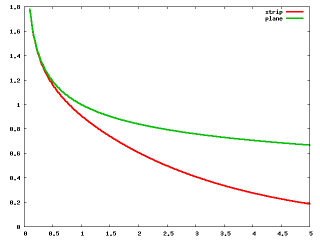 |
| Fig. 2: Ising correlators for strip vs. plane geometry, function of longitudinal distance. |
If the distance between the points is small compared to L, the correlation function reduces to the form for the infinite 2D geometry. On the other hand, if the distance is large compared to L, the correlator takes the form of a negative exponential, with length scale L/2π. Conformal invariance would forbid the existence of such a length scale in the fully infinite 2D case, but for the strip geometry, the length in the finite direction sets a natural length scale for the theory. The figure at right displays a plot of the correlation function in the strip geometry (L=2), in red, and the correlation function in the plane, in green. For small values of r, the two are equivalent, since the spins don't "know" what type of geometry they reside in. But for distances comparable to L, the correlator in the strip is exponentially suppressed with respect to the correlator in the plane. This can be understood as follows: for large separations along the strip, the geometry begins to "look" one dimensional. In 1D, there is no finite temperature phase transition in the Ising model, thus we expect an exponential decay in the correlations.
© 2007 D. Stanford. The author grants permission to copy, distribute and display this work in unaltered form, with attribution to the author, for noncommercial purposes only. All other rights, including commercial rights, are reserved to the author.
[1] J. Cardy, Scaling and Renormalization in Statistical Physics (Cambridge, 1996).