The Imaginary Time Propagation Method (ITP) has long been used as a way to find ground-state wavefunctions. [1] However, if one is only interested in the ground-state energy, a few tricks may be employed to reduce the computational burden. I describe here in particular a method whereby, for n particles with an arbitrary Coulombic potential, the analytical calculations may be done in a n-dimensional space instead of a 3n-dimensional space.
In general, finding the ground-state wavefunction directly from the Hamiltonian for a quantum system is a nightmare, with only a few known exactly-solvable systems. However, the Schrödinger equation yields to a cute mathematical trick, so that it is possible to approximate a ground state wavefunction to arbitrary accuracy. This trick, known as Imaginary Time Propagation (ITP), involves substituting imaginary time instead of real time into the time-dependent Schr7ouml;dinger equation. This leads to the derivation of an imaginary-time operator which results in exponential decay of all states except for the ground state, which can then be applied to any initial trial wavefunction to compute an approximation to the actual ground state.
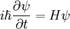
As mentioned, we begin with the time-dependent Schrödinger Equation:
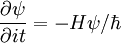
Equivalently, in terms of the derivative with respect to imaginary time, we find that
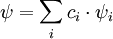
To see why this is useful, we first write ψ as a sum of eigenfunctions of the Hamiltonian H, where each eigenfunction ψi has corresponding energy Ei:
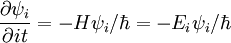
For each eigenfunction, the imaginary-time Schrödinger equation then becomes
The solution to this expression is an exponential. If we define

we find that

where as usual
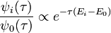
Evidently, when propagated forward in imaginary time, each eigenfunction decays exponentially, with the rate of decay proportional to its energy. Indeed, all the states other than the ground state will die off exponentially quickly even compared to how quickly the ground state is vanishing:
If we apply the solution for the eigenfunctions to the original wave function, we find
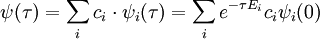
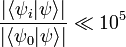
Hence, in the limit of imaginary time propagation, the coefficients for the scattering part of the wavefunction approach zero and those for bound states approach infinity. Note, however, that the relative proportion of the ground state wave function in the overall wave function always increases as a function of imaginary time because Ei > E0:
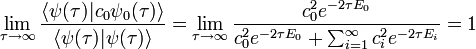
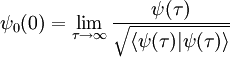
Thus, starting with any wavefunction ψ, we find that in the limit of large τ, the wavefunction will become proportional to the ground-state wavefunction:

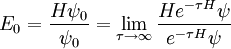
And, in particular, we may compute the ground-state wavefunction exactly, as long as the overlap c0 between our initial wavefunction and the ground-state wavefunction is nonzero:
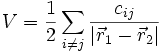
Full ITP normally involves numerically propagating a trial wavefunction for many time steps over a large volume in parameter space. If we are only interested in finding the ground-state energy of a system, this seems particularly wasteful. For an eigenfunction ψi of the Hamiltonian, it is true at any point in parameter space that Hψ0 = E0ψ0. This suggests a simple method for ITP at a single point. Suppose that in natural units our Hamiltonian for n particles is of the form
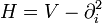
where, as usual,
 |
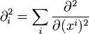 |
As rectilinear partial derivatives commute with themselves as well as partials with respect to imaginary time, we may then write down the equation for the imaginary time evolution of the derivatives of ψ:

Now, if we start with the initial value of ψ at a point and some large number of its derivatives, we can evolve both ψ and its derivatives according to the imaginary-time Schrodinger equation. After some appropriate amount of time, we can then extract the ground-state energy just by applying H to ψ at the particular point we have chosen.
However, this is not especially better than a brute-force solution. Even though derivatives commute, if there are n dimensions, there are
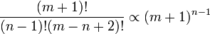
distinct ways to take m derivatives. While we would not have to worry about spatial boundary conditions, we would have to worry about "boundary" conditions on the derivatives which we choose not to propagate. Hence, we have simply mapped the complexity of the problem in a virtually one-to-one manner into a different (but no more useful) form.
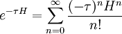
For a better approach, we recall the expression for the ITP of ψ, decomposed into eigenfunctions:

Evidently, if we can calculate the effect of the operator e − τH on ψ(0), we can immediately recover the ground-state energy:
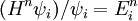
Then, we simply have to calculate a number of terms in the expansion of exp(- τH). How many? The answer naturally depends on the initial wave function ψ which we choose and the desired accuracy which we want. Suppose, for instance, we pick a wavefunction which is some (unknown) superposition of bound states and we desire an accuracy of one part in 109. We expect that (unless we get extremely unlucky with our choice) we will find
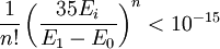
This would suggest that we would like exp[-τ(E10)] < 10-15, or, in other words, τ(E10) > ln(1015) ≈ 35. In that case, how fast does the series for exp(-τH) converge? If we note that
then
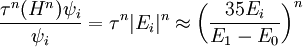
Thus, for our desired accuracy, we want
for i > 0. We expect this to be maximum for i = 1, if the states are ordered in terms of increasing energy. For Hydrogen, for instance, where 3E1 = (E1 - E0), this implies that about 56 terms in the expansion are necessary. For Helium, where 3(E0 - E1) ≈ E1 this would imply the calculation of 320 terms. If one had an estimate of E1, one could naturally take away E1 / 2 from the entire energy scale, dramatically reducing the number of terms necessary (38 terms for Hydrogen, 173 terms for Helium).
This, at least, sets a sensible upper bound on the size of the calculation. For any one-dimensional calculation, this method is clearly a fine choice---as each derivative in the Hamiltonian can only be taken one way, calculating each successive term in the expansion only requires that one derivative be taken. However, one-dimensional calculations are hardly impressive. In fact, up to the present time, we have gained no advantages by evaluating exp(-τH) ψ at a single point. Since a new Laplacian is applied for each term, we end up taking 2m derivatives to calculate m terms, resulting in a computational burden of about (2m)n-1 distinct derivatives at the final step.
While one could pick a simple initial wavefunction with simple derivatives (such as ψ(0) = exp(-r)), this does not help matters. Observe, for example,

The last term is the trouble, for it means that no matter how simple our wavefunction is, we still end up calculating derivatives of V and, by extension, V2, V3, and so on.
Nonetheless, with certain potentials, the derivatives of Vn can still end up taking extremely simple forms. One case in point is Coulombic potentials, where
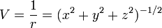
Most obviously, ∇2 = 0 (except at certain points) which reduces the number of distinct derivatives one must calculate. However, there's a more subtle consideration which is much more important. Consider a two-particle potential, with one particle at the origin:
If we evaluate exp(-τH) ψ at the point (x,y,z) = (0,0,1), then any elements of our answer which involve positive powers of x or y will evaluate to zero, and we can skip calculating them entirely. Indeed, as it turns out, we can skip calculating derivatives with respect to x entirely until the very end of our calculation, because they all take a very simple form. In particular, we can make a simple table of even derivatives, noting that all odd derivatives will evaluate to zero at x = 0:


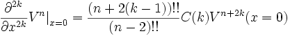
where C(k) is a simple function purely depending on k:
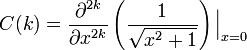
and where m!! is the semifactorial


Evidently, we can apply this to derivatives with respect to y, where we find

Or, in general, if we need to make up m total derivatives this way, we find

where
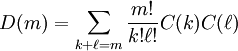
If, for whatever reason, we are examining the two-particle system in higher-dimensional spacetime, then further coefficients in the style of D(m) are no harder to calculate:

So that calculations of this type are linear in terms of the number of dimensions involved.
Hence, we may treat this as a purely one-dimensional problem, taking only derivatives with respect to z, and then only at the very end taking derivatives with respect to x and y as necessary to round out the Laplacians. That is to say, the effect of adding extra dimensions is a purely combinatorical factor multiplying the final result. Now, of course, this should not be impressive yet - after all we started with a 1D-potential, namely V = 1 / r.
However, with more particles, this trick - namely, that the derivatives all take the same general form - becomes astoundingly useful. We cannot expect to place all the particles on top of each other, obviously. Nonetheless, in problems where the particle locations are not constrained, we choose to evaluate exp(-τH) ψ at a location in parameter space where all the particles are lined up in a straight line along the z-axis. That is to say, xi = yi = 0 for each particle, so that (xi - xj) = 0 and yi - yj = 0 for any pair of particles. Then, we find that the only nontrivial derivatives in the expansion of exp(-τH) - i.e., terms which are not purely powers of the distances between particles - result from derivatives with respect to the particle locations on the z-axis. At the end, we may apply the effects of the extra dimensions all at once - as they cannot result in new terms, and as they only result in multiplication by a simply-calculable number, their computational cost becomes linear in the number of nontrivial derivatives already calculated.
Consequently, we have reduced a 3n-dimensional problem to a n-dimensional problem. Hydrogen, as before, remains a 1D-problem; Helium becomes a 2D problem; Lithium becomes a 3D problem, and so on and so forth.
In the previous section, we only considered fixing the locations of particles in two dimensions each. We consider it likely that by (for example) fixing particles to be at a constant spacing along the z- axis, it may be possible write all the derivatives along the z - axis in terms of each other - resulting in the derivative of only one dimension being unique. This would be truly satisfying - as energy is a single-dimensional quantity - we would then be at a minimum of work required to calculate it.
© 2008 P. Behroozi. The author grants permission to copy, distribute and display this work in unaltered form, with attribution to the author, for noncommercial purposes only. All other rights, including commercial rights, are reserved to the author.
[1] W. Magnus, Comm. Pure Appl. Math. 7, 649-673 (1954).