|
|
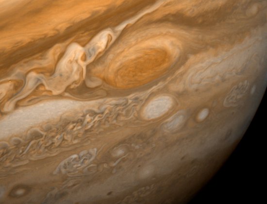
| Fig. 1: Closeup of Jupiter's Great Red Spot. (Courtesy of NASA/JPL-Caltech) |
The great red spot of Jupiter (GRS), a 14,000 by 40,000 km elliptical anti-cyclonic vortex, has persisted for hundreds of years of continuous observation despite the highly turbulent jovian atmosphere. At first, scientists believed the GRS was attached to some topological feature on the surface of the planet. But in 1970, G. S. Golitsyn suggested that the GRS is a free vortex independent of any solid feature, which arises from the unique conditions on Jupiter: a large coriolis force arising from the planet's rapid rotation; a thin, inviscid, weather layer; and wide, azimuthal, axisymmetric regions of cyclonic and anticyclonic shear [2].
Then, the NASA Voyager missions of the 1970s showed that the GRS is localized in latitude (~22°S), but drifts azimuthally around the planet. This observation confirmed the free vortex theory, and theorists began putting forth geophysical hydrodynamic models to capture the GRS's essential features, including anti-cyclonic flow, high stability in the face of dissipation and dispersion, a 2:1 aspect ratio, and the swallowing up of smaller vortices by bigger ones. This study of the GRS led to substantial progress in the field of geophysical fluid dynamics, and has given us a better understanding of earth's atmosphere and oceans in the process. Further, the techniques have been applied to other vortex systems such as pure-electron plasmas [3].
| Jovian Rotational Velocity | Ω≅1.7*10-4sec-1 |
| Length Over Which Speed Varies | L≅104 km |
| Characteristic Speed of Motion | U≅50 m/sec |
| Rossby Number | ε = U/2ΩL ≅ .015 |
Some models propose that the jovian atmosphere is somewhat viscous, and that the surface features we see are part of a system in which the weather layer moves with the deep atmosphere, which in turn is driven by internal heating [4]. Were this the case, understanding the physics behind the GSR would be impossible without observational data of the deep jovian atmosphere. However, density data obtained from the outermost layers of the jovian atmosphere show that the cloud tops of Jupiter act more like a frictionless layer of water superposed on an independent, time-invariant stream function. The best model for this situation is the rotating shallow-water equation. We begin with the conservation of momentum and mass for an inviscid, incompressible fluid element, in which the horizontal velocity is approximately independent of z, the local normal direction:
Where f(y) is the coriolis parameter, a function of the latitude. Taking the curl of the first equation and combining it with the second, one can show that
Where ω(x,y,t) is the relative vorticity, the curl of the horizontal velocity field [1]. It is standard to call the advectively conserved quantity ωp = H0(ω(x,y,t)+f(y))/H the potential vorticity.
Finally, it is standard to employ the β-plane approximation, which says that for motions sufficiently small in the north-south direction, one can treat the coriolis force as varying linearly with the locally flat north-south coordinate y,
Where the linearization is about some mean latitude Θ0. Depending on the scales between the horizontal motion, the vertical motion, and the planetary rotation, it is possible to expand this potential vorticity as a power series in the Rossby number, ε = U/(f0L), and keep only those terms which contribute.
The shallow-water potential vorticity equation becomes easier to compute numerically when made advectively linear by an approximation scheme based on the scalings of flow. For Jupiter, ε ≅ .015 (see Table 1). This motivates the quasi-geostrophic (QG) approximation, which expands the shallow-water equation to first order in ε, resulting in the kinematic geostrophic balance equation,
Where v is a function of the stream function ψ = gh/f0 [1]. Employing both the QG approximation and the β-plane approximation, Marcus derived from this a form for the potential vorticity in cylindrical coordinates [5].
Where ψ is the stream function of the weather layer, ψlower is the stream function of the underlying atmosphere, and LR the radius of deformation, a measure of the stratification of the planet. The underlying stream function is assumed to be time independent compared to the dynamics of the the GRS (e.g. measured by its turn-around time).
The advective conservation of this form of the potential vorticity was numerically solved by spectral methods [5]. The striking result of the simulation is that the stability of large vortices is made possible by their constant "swallowing up" of potential vorticity from smaller vortices. This may explain both the interaction of jovian vortices and the long lifetimes of the largest ones, such as the GRS. Further, the simulations show that for an azimuthal axisymmetric underlying stream function (which varies with latitude), all stable vortices are prograde (their vorticity has the same sign as the local shear). This matches the observation that jovian vortices can be cyclonic or anti-cyclonic, as long as they match the local zonal shear. The GRS's 2:1 aspect ratio is explained as a case when a single vortex has more vorticity than can be fit between the boundaries of its local zone, forcing it to elongate. The QG model gave rise to vorticity profiles peaked around the edges of circulations, with relatively low velocities in the center, which also matches observational data.
Marcus followed up this work by adding a forcing and dissipative term into the potential vorticity equation,
Where F represents forcing due to the underlying layer, e.g. convective overshoot [6]. The systems was now initialized with the entire atmosphere at rest, and for a certain set of forcing and dissipative parameters the persistent vortices and the zonal flows were shown to arise from the QG approximation.
Sommeria et al. created a laboratory simulation of the QG regime by a rapidly rotating annular tank, with a stream function generated by input and output holes in the bottom of the tank [7]. They recreated the beta-effect (the spatial variation of the coriolis force) by using a sloped bottom. As the tank speed increased, the number of stable vortices decreased until there was a single persistent vortex that exhibited the vortex-merging behavior discussed above. Such experiments had been previously performed, but this was the first to use large enough tank rotational velocity to achieve a Rossby parameter small enough to be comperable to Jupiter. Their setup may be critiqued as non-axisymmetric (they had six pairs of localized input and output holes through which pumping occured). However, when paired with the numerical simulations of Marcus, QG dynamics paint a convincing picture of the GRS.
Solitons are persistent solitary waves of finite amplitude in a dispersive medium. They often arise as solutions of the Korteweg-de Vries (KdV) equation,
A PDE describing dissipative, dispersive waves in a medium of finite depth that provides a nonlinear restoring force. When the dispersive term balances the nonlinear divergent term, weakly interacting, stable solutions results. Solitons are an appealing GRS model because they are persistent despite a dispersive environment by definition. The first major theoretical papers proposed to explain the stability of the GRS came in this form, examining the shallow-water equation under the condition that wave-length is comparable to layer height, to obtain a KdV equation. The work of Maxworth and Redekopp begins with the QG approximation and examines motions that consists of a mean zonal flow and a perturbation of the order of the Rossby number, ε [8]. They begin with a form of the QG potential vorticity equation,
Where N is the Brunt-Vaisala, or boyancy frequency, and is related to the deformation radius by LR = NH/f0. Then he assumes that the stream function consists of a mean zonal flow U(y) and a disturbance of order ε to rewrite this as

He shows that this equation supports soliton solutions of the form,

Provided that the amplitude function of the circulation obeys a modified KdV equation (the nonlinear term becomes quadratic)
Where τ and ξ are rescaled time and space coordinates. Further, when the situation lacks baroclinicity (see next section), the modified KdV equation reduces to an ordinary KdV equation. As already mentioned, these solutions are appealing because they are by nature stable, dispite the dispersion caused by a space-varying coriolis force. The work of Williams also uses soliton solutions to model the GRS, but disputes the scaling arguments leading to the QG approximation for the GRS, and instead favors an intermediate-geostrophic (IG) approximation [9].
However there are drawbacks to these models. Solitons have the characteristic of emerging from soliton-soliton interactions unchanged except for a spatial phase shift, unlike the behavior of jovian vortices. And in the case of William's IG solitons, a gaussian vorticity profile emerges which is unlike the calm center of the actual GRS. Soliton vortices have been produced in a laboratory by rotation of an annular tank with a parabolic bottom, but the resulting vortices did not take on the characteristic elongated shape and interacted far more weakly with small vortices when compared with the GSR [10].
Baroclinicity refers to a misalignment of surfaces of constant pressure and constant density. When the surface of a planet is subject to differential heating such that the temperature gradient is a nonlinear function of distance, baroclinic instabilities result which may lead to the formation of stably eddies. Read suggests the persistent jovian vortices may be baroclinic eddies, driven by the transport of heat between the edges of their zonal flows [11]. He begins with the QG potential vorticity equation, but includes an additional forcing term that accounts for the thermal structure of the flow in the form.
Read also created a laboratory analogue of this model [12]. By heating and cooling the sidewalls of a rotating annulus filled with fluid, slantwise convection emerged which did lead to stable eddies. However, in the case of Jupiter, the cause of such a the temperature gradient would be unknown, and the vortices can exist only in a range near laminar flow, whereas the flow on Jupiter is turbulent. That is, while baroclinicity may play an important role in planetary vortex systems, its role in describing the GRS is not fully motivated. Further, the work of Philip Marcus, which proceeded this work, was able to show the emergence of stable, robust vortices with a more minimal set of assumptions.
A series of theoretical studies have been performed over the past three decades to capture the essential features of the GRS, and in particular its long lifetime, while making the minimal number of unmotivated assumptions. The simplest assumption, that the GRS is attached to some solid feature, gave way to free vortex hydrodynamic theories. Baroclinic eddies arising from the transport of heat across zonal boundaries could account for the GRS, but it is unclear how such a situation would arise. Soliton solution to geostropic equations of motion too could explain the longevity of the GRS, but they do not capture the way it merges with smaller vortices. Using only the QG and β-plane approximation, Marcus demonstrated not only the persistent vortices, but the zonal flows themselves, as emergent phenomena. While the resulting model does not capture every minute detail of the GRS, a deeper model may require further observational data to be motivated.
© 2007 Michael Jeremy Rosen. The author grants permission to copy, distribute and display this work in unaltered form, with attribution to the author, for noncommercial purposes only. All other rights, including commercial rights, are reserved to the author.
[1] M. Ghil and S. Childress, Topics in Geophysical Fluid Dynamics: Atmospheric Dynamics, Dynamo Theory, and Climate Dynamics (Springer-Verlag, 1987).
[2] G. S. Golitsyn, Icarus 13, 1 (1970).
[3] P. S. Marcus, T. Kundu and C. Lee, Phys. Plasmas 7, 5 (2000).
[4] F. H. Busse, Geophys. Astrophys. Fluid Dyn. 23, 153 (1983).
[5] P. S. Marcus, Nature 331, 693 (1988).
[6] P. S. Marcus and C. Lee, Chaos 4, 2 (1994).
[7] J. Sommeria, S.D. Meyers and H.L. Swinney, Nature 331, 689 (1988).
[8] T. Maxworthy and L. G. Redekopp, Icarus 29, 261 (1976).
[9] G. P. Williams, Adv. Geophys. A 28, 381 (1985).
[10] S. V. Antipov, M. V. Nezlin, E. N. Snezhkin, and A. S. Trubnikov, Nature 323, 238 (1986).
[11] P. L. Read and R. Hide, Nature 308, 45 (1984).
[12] ibid., Nature 302, 126 (1983).