|
|
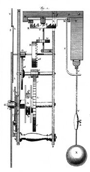
| Fig. 1: A schematic for Huygens' pendulum clock. This figure is currently under a free license as stated here. |
Christiaan Huygens, a Dutch scientist, invented the pendulum clock in 1657[1]. Until his invention of the accurate clock, the matter of timekeeping hindered advances in many fields of science and expeditions. An accurate timekeeping method can enable the precise measurement in Physics, as well as the applications in daily life. In addition, the Europe was entering "the age of exploration," which required explicit time measurement for the maritime voyage[2]. Although Galileo Galilei studied the mechanism of the pendulum and conceived the pendulum clock concept, no clock using the periodicity of pendulum was demonstrated. The problem to realize a clock from the physical concept was the period of pendulum varies when the pendulum makes wide swing. To regulate the swing of the pendulum, Huygens introduced a kind of escapement and cycloidal confinement of a flexible pendulum suspension, which is isochronous curve. In consequence, Huygens made a clock of which error was under 10 seconds a day. It was a great breakthrough in time measurement, compared with the previous limit - 15 minutes a day.
However, accurate regulation of the pendulum period was not the whole work from the pendulum clock. After combining two nearly identical pendulum clock in same support, Huygens discovered the "odd sympathy." [3]
| "Of an odd kind of sympathy perceived by him in these watches (two maritime clocks) suspended by the side of each other."[4] |
Huygens saw that the two suspended pendulum's motion became the state of same frequency and exactly opposite direction, regardless of the initial condition. Even after he disturbed one pendulum, the system was back to the "antiphase state." At first, he thought that the reason was interference between two pendulums via air flow. But after several experiment, he concluded that the insensible movements and mechanical interaction on the frame caused the coincidence in motion.
The Huygens' experiment inspired the following studies of interacting nonlinear oscillators. The topic is basically of two mechanical oscillator with weak coupling, but it's notion of synchronization widely affected various problems from nonlinear dynamics to complex biological system. [5] In physics, the coupling of two oscillators are rediscoverd by novel magnetic and mechanical systems of nanometer scale. [6,7]
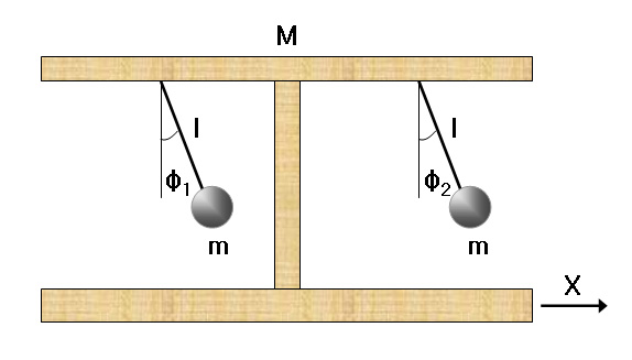 |
| Fig. 2: Basic model for two coupled oscillator system. |
Even though the synchronization in coupled pendulum have been known for over 300 years, the attempts to solve the phenomena were not quite satisfactory. [8,9] Recently, researchers from the Georgia Institute of Technology (Bennett et al.) tried to reexamined the old experiment both in experimental and theoretical ways. [10]
Fig. 2 shows the simplified schematic of the coupled pendulums. Each pendulum consists of an identical point mass m and a massless rigid rod with equal length l. φk is the angular displacement of the kth pendulum about its own pivot point. And X is the linear displacement of the system's center of mass. To simplify the discussion, we can assume that the mass of platform M is much larger than the point mass m. It also means that the coupling between two equal mass is a weak coupling, since the effect of one pendulum's motion is small compared to the inertial of the frame - which transmits the coupling between two identical masses.
To solve such complex system analytically first, we start from the system without damping term and driving terms. With the basic assumption, the Lagrangian will be
Here we use the term of K, since the original experiment conducted by Huygens was settled on rest frame. However, further experiments reveals that the term only makes minor effect in the result. [10] And now we introduce viscous damping term for both angular motion and translational motion, as well as the driving term from the escapements. Then the equation of the motion become
where b is a damping coefficient for swinging and B is a damping coefficient of translational motion. With the small angle approximation and impulse-free condition, we can express the characteristic equation of the system. It is convenient that the variables are scaled as dimensionless forms. When we write the equation with two variables σ = φ1 + φ2 and δ = φ1 - φ2, the equations are
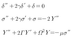
where Y = X/l, γ = b (l/4g)1/2, Γ = B (l/4g)1/2/(M+2m), Ω2 = K/(M+2m), μ = m/(M+2m), and the prime means differentiation with respect to τ = t(g/l)1/2. The system mass ration μ indicates the magnitude of the coupling. And with the later discussion, we can figure out that the value of μ does important role to determine the overall behavior.
 |
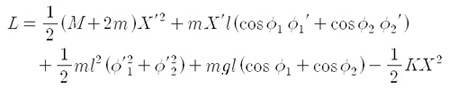
| Fig. 3: The "truncated" phase diagram of single pendulum with periodic impulse. |
One important feature is derived from above equations. Let's compare the differential equations of σ and of δ. For the extreme case with no viscous damping(γ = 0),σ would damp out due to the Y'' term. That is, among two different modes of pendulums, antiphase mode(δ) survives at last whereas inphase mode(σ) vanishes. Although this analysis is induced with the condition between periodic kicking - no external impulse, the characteristic of the mode is valid after the simulation considering the energy input.
Until now, we only treat the isolated system from the outside driving. In order to consider the energy input, it requires the normal mode evolutions and the analysis of nonlinear Poincare section. I will not discuss the details of the works done by Bennet and the much since it includes numerical analysis with several strong restrictions to converge the calculation. The brief strategy is following; at first, we can derive the normal modes and neglect one mode since we assume that "imperceptible movement - weak coupling." And among the four dimensional phase space, we can focus just on three dimensional map. In addition, for counting outside impact, we introduce the "truncated" orbit in phase space due to the forced change of the pendulum movement (Fig. 3). With the consideration of both damping and energy input, the numerical simulation shows that the three dimensional map reveals two stable states and one unstable state asymptotically. Two stable states are antiphase state(φ1 = - φ2) and the trivial state, whereas the inphase state(φ1 = φ2) is unstable. [10] This is a consistent with Huygens' observation.
 |
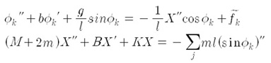
| Fig. 4: Phase diagram from the theoretical simulation: (a)Δ - μ plane with Γ fixing (b)Γ - μ plane with Δ fixing. |
One last thing we should consider is that the non-identical condition of two pendulums in real experiment. Therefore, we also need to verify in what condition such antiphase collapse in terms of the difference between two pendulums. The difference is represented by the "detuning" variable Δ, which is accounted for the difference in pendulum frequencies. And with the previous constriction for the simulation, the critical detuning Δc is given as the below expression.
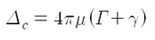
Fig. 4. describes the overall conditions determining the system's behavior. There are three parts in each phase diagram. Quasiperiodic domain means two forced pendulum do periodic motion with different frequency. And in the 'Beating Death' domain, one of the pendulum stops to move even the other pendulum swings periodically. The antiphase mode survives only with the proper condition - nearly identical conditions and intermediate relative magnitudes of the damping and the coupling terms. Fortunately, Huygens' clock satisfies all of the conditions above; so that the secret of 'sympathy' in nature comes out to us finally.
© 2007 Seung Sae Hong. The author grants permission to copy, distribute and display this work in unaltered form, with attribution to the author, for noncommercial purposes only. All other rights, including commercial rights, are reserved to the author.
[1] C. Huygens, The Pendulum Clock or Geometrical Demonstrations Concerning the Motion of Pendula as Applied to Clocks, ed. by R. Blackwell (Iowa State University Press, 1986).
[2] J. G. Yoder, Unrolling Time: Christiaan Huygens and the Mathematization of Nature (Cambridge, 1990).
[3] C. Huygens, Oeuvres Completes de Christiaan Huygens, ed.by M. Nijhoff (Societe Hollandaise des Sciences, 1893).
[4] T. Birch, Philosophical Transactions vol. 2. (Johnson Reprint, 1968), p. 19.
[5] J. Buck and E. Buck, Science 159, 1319 (1968).
[6] S. Kaka et al., Nature 437, 389 (2005).
[7] F. B. Mancoff et al., Nature 437, 393 (2005).
[8] D. J. Korteweg, Les Horloges Sympathiques de Huygens Serie II. Tome XI, ed. by M. Nijhoff (Archives Neerlandaises, 1906), p. 273.
[9] I. I. Blekhman, Synchronization in Science and Technology (ASME Press, 1988).
[10] M. Bennett et al., Proc. R. Soc. London A 458, 563 (2002).