WARNING TO BACTERIA: If you happen to be a bacteria looking for some breakfast, watch out for tightly focused lased beams in your path! And if you are unlucky enough to run into one, you'lll have quite a time trying to run away from it - it'll pull you back with an enormous force of the order of pico Newtons. Not only that, the grad student controlling the laser beam can even move you around at will by moving the position of the laser spot. Well, given that you are reading my report, you are more likely to be the grad student, or someone interested in how grad students tease bacteria and not the bacteria itself. In what follows, I shall attempt to give a simple description of the workings of an Optical Tweezer, so that you are ready to tease the next unfortunate bacteria you meet!
A tightly focused laser spot generates around it a harmonic potential, where particles whose sizes are more than a particular threshold (typically ~ microns), and whose refractive indices are more than that of the surrounding fluid can be mechanically confined. This arrangement is called an optical tweezer, and the maximum force that an optical tweezer typically generated is ~ pN. Proper treatment of an optical tweezer depends on how the size of the particle is, relative to the wavelength of light used. If the particle size is much greater than the wavelength, we are in the regime of ray optics, and if the particle size is much smaller compared to the wavelength, the conditions of Rayleigh scattering is satisfied, and the particle must be treated as a point dipole.
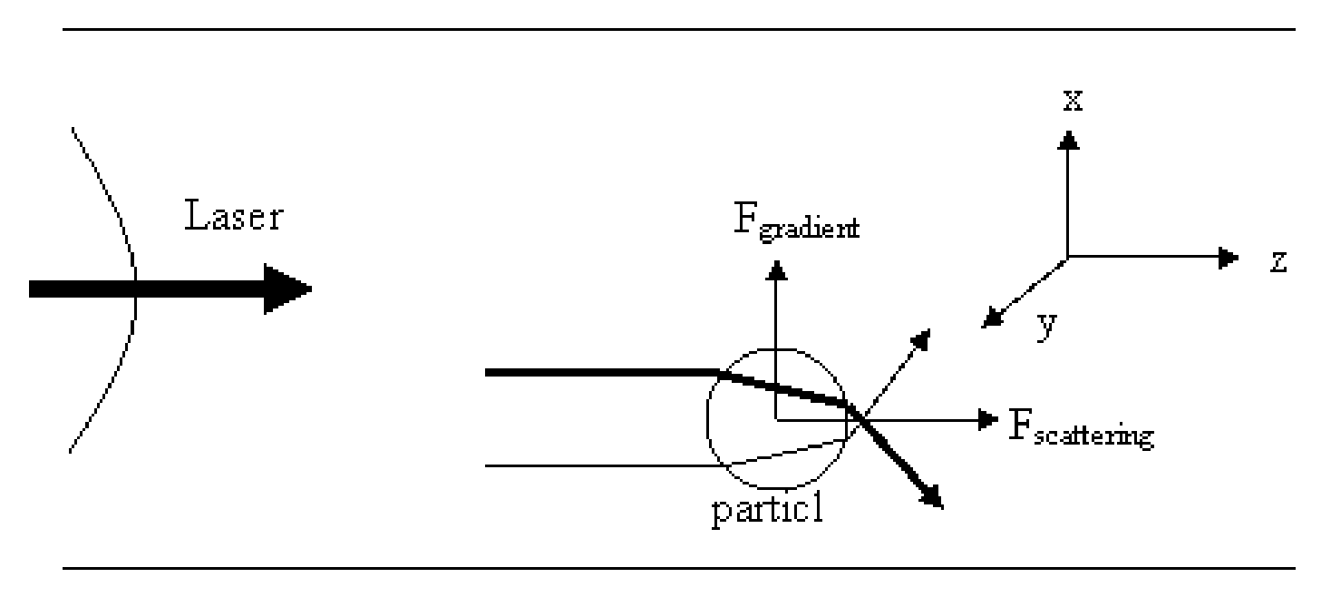
A particle in the path of a beam of light feels two types of forces. The first is a scattering force arising due to reflection of photons off the surface of the particle. This tends to push the particle in the direction of the beam. The other force, called the gradient force, arising due to refraction of photons through the particle, tends to pull the particle towards regions of higher intensity. To understand the origins of these forces, let us turn out attention to figure 1, which shows a particle in the presence of a lased beam with a Gaussian intensity profile.
|
|
| Fig. 1: Caption goes here. |
In figure 1, we follow two rays refracting through the particle. The one drawn in bold has more intensity than the other ray shown, as the bold ray is closer to the center of the laser beam. The photon traversing along the weaker ray feels a momentum change in the x direction (and -z direction), and hence a force in the x (and -z) direction. Similarly the photon traversing along the bold ray, feels a force in the -x (and -z) direction, and hence a force in the -x (and -z) directions. These, by Newton's Third Law, cause the particle itself to feel a force, in the -x and z directions (due to the photon along the weak ray) and x and z directions due to the photon along the bolder ray. But since the number of photons traversing per unit time along the bold ray is more than that along the weak ray, the particle feels a net force in the x direction (labeled as Fgradient) and a net force in the z direction (labeled as Fscattering). As we can see from this simple picture, Fgradient tends to pull the particle towards the center of the beam, that is, towards the region of high intensity. Fscattering tends to move the particle along the beam, and reflection off the surface of the particle also contribute to (and actually dominate) Fscattering.
This arrangement does not really trap the particle - rather, just guides the particle along the laser beam. Ashkin, in 1970, first observed this phenomenon by guiding small polystyrene beads along a laser, and even steering them around by steering the beam [1]. So how can we trap the particle, that is, cancel out the scattering force? The first solution would be to simply use two counter propagating beams, which would cancel out the Fscattering, and each beam would stabilize the particle towards the central axis. Ashkin was the first to construct such a dual beam optical trap [1]. But this arrangement is extremely complicated in terms of alignment (as the optical axes have to coincide), and moving the two beams around together is difficult.
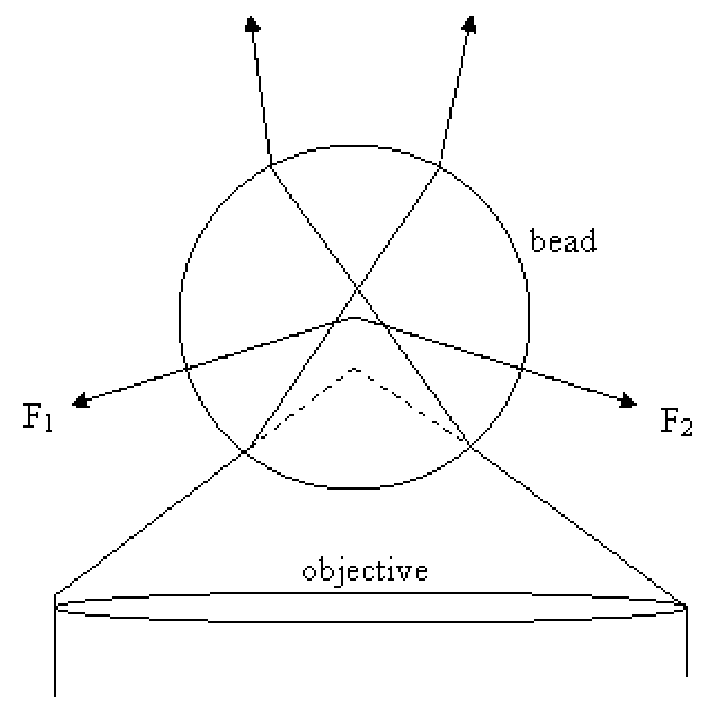
To overcome this problem, optical tweezers of today rely on just one beam. The idea is a simple extension of the scheme described above, and involves creating a strong intensity gradient along the direction of the direction of the beam as well (i.e. along the x axis in Figure 1). Ashkin again, in 1986, was the first to create this, by using a tightly focused laser spot, which of course creates a strong intensity gradient along the z direction [2]. The scattering force is still present, but is far dominated by the gradient force if the particle being trapped has a low enough reflectivity. Equilibrium is finally achieved a bit above the focal spot, where the scattering force and the gradient force balance. Figure 2 explains this geometry.
 |
| Fig. 2: Caption goes here. |
In figure 2, the dotted lines indicate the path rays 1 and 2 would have taken in absence of the bead. It is thus evident that F1 and F2 and the direction of forces that the bead experiences owing to photons along rays 1 and 2 changing the direction of their momentum while refracting through the bead. These forces thus combine to pull the bead towards to point where the rays would have come to focus, had the bead not been there (i.e., towards the point of intersection of the dotted lines). Of course, there is a scattering force as well, arising owing to the fact that some photons are reflected off the surface of the bead, but these are negligible if the bead does not have a high reflectivity. Finally, the particle comes to equilibrium a bit above the focus, where the scattering force and the gradient force balance.
As seen from figure 2, every photon impinging on the particle suffers a momentum change. Now, the magnitude of momentum of every photon remains constant, and equal to h/λ. The actual momentum change occurs owing to change in direction, and this depends on the location of the initial trajectory of the photon with respect to the optical axis. Say for a particular photon, the momentum change is Δp. Hence, change in momentum of the bead owing to refraction of that photon is -Δp. Now, the beam is assumed to be Gaussian, and completely defined by two parameters: (i) the distance from the center, x, where the intensity falls to I0/2, and (ii) the total integrated power W.

At r=x and I=I0/2, this gives g=ln(2)/z2. The other condition is the total integrated power:

This gives I0 = gW/π, which fully defines the beam. The other quantity is the lens stop, that is, the amount of light let in by the objective. This is basically equal to the back diameter of the objective. Now consider a patch on the plane of the objective at (r,φ). The number of photons passing per unit time through this patch is λI0/hc exp(-gr2) r drdφ. Hence, the force exerted on the bead owing to change in momentum of photons which pass the objective through the patch at (r,&phi) is given by

But, the magnitude of momentum does not change. Owing to this, we have

As this increment can be calculated for every (r,φ) by Snell's Law, this expression can be integrated over the entire objective to get the full trapping force.
In cases when the radius of the particle is significantly smaller compared to the wavelength of light, the conditions for Rayleigh scattering are satisfied and the particle can be treated as a point dipole in an inhomogeneous electromagnetic field. We consider a dipole formed by charges q and -q, located at locations r1 and r2. We define dx = r1-r2. Hence, the dipole moment p is given by q dx. The total force on it is given by

Now if we assume that the dielectric particle is linear, i.e. p=αE, then we have

Now we use the vector identity

and Maxwell's Equation

to obtain

ExB is proportional to the Poynting Vector, or the Intensity of the laser. Now, the frequency of the laser light is generally much greater than the frequency over which we are sampling, and hence the time derivative term in (2) averages to zero. We thus have

The square of the electric field is proportional to the intensity, and hence, we see that the force the dipole experience is proportional to the gradient of intensity, and hence directed towards the region of higher intensity. This is the origin of the gradient force. It's called the ponderomotive force, which is the force a charged particle experiences in a rapidly oscillating inhomogeneous electromagnetic field.
The above discussion motivates why a tightly focused laser spot should pull particles whose refractive index is less than that of the surrounding fluid, towards the point of equilibrium (which is slightly above the focal spot). Near the equilibrium point, any potential can be approximated as a harmonic potential, and so the next obvious question is how we can estimate the stiffness k of this optically generated harmonic potential. Now, if we experimentally measure the x position of the particle, we can compute ⟨x(t)2⟩. Now by applying the equipartition theorem

This formula can thus be used to calculate the stiffness of the trap. [3]
Here, I shall present a method, where the optical tweezer can be used as a viscosity probe, based on the power spectrum of the trapped particle. To do this, let us write Newton's law for a trapped bead

η(t) is the thermal noise term, arising owing to random thermal kicks the bead experiences. Since this noise is completely uncorrelated, i.e. "white", its power spectrum is a constant (2D). Also, as the mass of the bead is negligible, we can drop the inertia term, i.e. the system is over damped. Taking a Fourier transform, we have

Hence, the power spectrum is given by:

The stiffness k is obtained by fitting the experimentally obtained power spectrum to the Lorentzian. We obtain the damping coefficient γ=6πηa, where a is the radius of the particle and η is the local viscosity. Thus, an optical tweezer can be used as a local viscosity probe, and this has many applications in Rheology [7] and Biophysics.
Since Ashkin first reported Optical tweezing in 1970 [1], optical tweezers have found tremendous applications in Single Molecule Biophysics, as means of applying force, making mechanical measurements on, and manipulating single macromolecules or cells [4,5]. For these experiments, typically the biomolecule is attached to a bead (about a micron in diameter), which is then placed in the well of the trap, and can thus be moved around by moving the laser spot. The bead thus provides a mechanical handle, which can be pulled, twisted or in other ways, manipulated by the trap to detect the mechanical response of the biological sample. A major use of optical trapping has been in studying motor proteins [6], which are macromolecules that move within the cell, transporting cargo, or performing other functions. These proteins typically apply forces, which can thus be measured by measuring the opposing force an optical tweezer must apply to stall the motion.
At Stanford University, several groups have, over the years, developed single molecule techniques such as Optical Tweezers and magnetic tweezers, to study biological macromlecules. Steven Block's group [8] was the first to observe the 8 nm step size of the motor Kinesin, as it carries cargo from the central regions to the periphery of the cell [9]. James Spudich's Lab [10] has mastered the technique for studying the motor protein Myosin, which is responsible for muscle contraction. Currently, Zev Bryant's [11] group is developing single molecule techniques, such as magnetic and optical tweezers, to study DNA gyrase, which is a bacterial motor that applies negative supercoiling to DNA, and also to study myosin.
© 2007 Aakash Basu. The author grants permission to copy, distribute and display this work in unaltered form, with attributation to the author, for noncommercial purposes only. All other rights, including commercial rights, are reserved to the author.
[1] A. Ashkin, "Accelaration and Trapping of Particles by Radiation Pressure," Phys. Rev. Lett. 24, 156 (1970).
[2] A. Ashkin, J. M. Dziedzic, J. E. Bjorkholm and S. Chu, Opt. Lett. 11, 288 (1986).
[3] G. V.Soni, F. M. Hameed, T. Roopa and G. V. Shivashankar, Current Science, 83, 12, (2002).
[4] K. Svoboda and S. M. Block, "Biological applications of Optical Forces," Ann. Rev. Biophys. Biomol. Struct. 23, 247 (1994).
[5] R. M. Simmons, J. T. Finer, S. Chu and J. A. Spudich J. A. 1996. "Quantitative Measurements of Force and Displacement Using an Optical Trap," Biophys. J. 70, 1822 (1996).
[6] C. Wigging, "Optical Trapping Interferometry Study of Molecular Motor Kinetics," Thesis, Department of Physics, Joseph Henry Laboratories, Advisor: Steven Block.
[7] A. Meyer, A. Marshall, B. G. Bush and E. M. Frust, "Laser Tweezer Microrheology of a Colloidal Suspension," J. Rheol. 50, 77 (2006).
[9] K. Svoboda, C. F. Schmidt, B. J. Schnapp and S. M. Block, "Direct Observation of Kinesin Stepping by Optical Trapping Interferometry," Nature, 365, 721 (1993).
[10] http://biochem.stanford.edu/spudich/
[11] http://med.stanford.edu/profiles/bioengineering/faculty/Zev_Bryant/